4 Using R Effectively
There are many things you can do to set yourself up for success and make your life easier (both now and in the future). It is really important to start implementing these good practices ASAP to establish good habits early on. It is much harder to break routines later. Both coding best practices in general as well as some things specific to R and RStudio will be covered below.
Remember the quote mentioned previously:
You are always working with at least one collaborator: Future you.”
-Hadley Wickham
Even if for selfish purposes only, and you ignore how this could impact anyone else, help future you. Do not put future you in a position where they are mad at present you!
4.1 RStudio
4.1.1 Settings
There are a number of settings tweaks that you will want to make to help force you into some good habits.
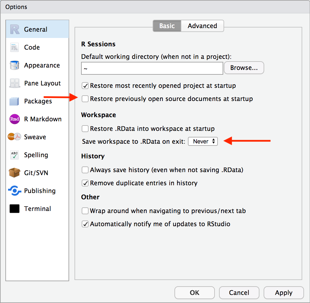
- “Restore .RData into workspace at startup” is unselected
- This will make RStudio load the .RData file (if any) found in the initial working directory into the R workspace (global environment) at startup.
- “Save workspace to .RData on exit” is set to Never
- Ask whether to save .RData on exit, always save it, or never save it.
These basically just make it so that variables and other saved data floating around in your global environment get preserved and automatically loaded if R closes. This can create an over-reliance on things that just exist locally in your files. This is very much contra to the whole aim and benefit of reproducibility by using R! You should always be able to easily re-run your code and get anything you need.
It can also cause weird behavior in between your R sessions because some things may still be saved in your workspace and you do not realize it.
It is thus best practice to not feel attached at all to the stuff in your workspace. If you need something, rerun your code to get it! If you have things that you think would be hard to replicate, that is a problem you need to fix!
Particularly because most of the time you cannot predict when things will go wrong…

Artwork by Horst (2022)
The settings changes above help fix this. Something else that you can do yourself is to regularly restart R, clear all content, and re-run your code scripts (particularly if they are in development!). You can restart R from the Session menu, or the keyboard shortcut cmd/ctrl+shift+F10. You can clear your workspace and output by using the brooms!

Upper right pane: click on environment tab, then click on the broom
Lower left pane: in console tab (at the top right), click on the broom too
One other settings change to make is:
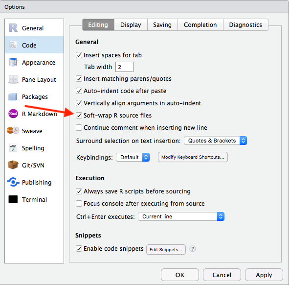
- “Soft-wrap R source files” is selected
- This will just make some of your written code easier to read, so you will not have to scroll horizontally. This only impacts working in RStudio, not your outputs!
Full explanation of the different RStudio settings can be found here.
4.2 Functions
“To understand computations in R, two slogans are helpful: Everything that exists is an object, and Everything that happens is a function call.”
- John Chambers, Advanced R, p. 79.
You have already used a few functions before (typeof(), class(), here()), but they will be formally introduced now. Almost everything you do with coding is built around using functions. Functions are variables containing pre-written code which, most often, have a verb name and are always followed by a set of parentheses. The things inside the parentheses, called arguments, are what that verb will be applied. When running:
typeof(x = myDF)
You are finding what type myDF is. This function has one argument, x, that is given the value “myDF”. Functions expect arguments to be given values. They need something to apply the pre-written code to! Functions that have multiple arguments often have default values, so you only need to set one or a few of them. you will see more about this later on.
Note: Arguments are separated with a comma and should often be given their own line.
4.2.1 Where Do Functions Come From?
A number of different sources! They are:
- Available from base R
- By default, R has many functions (like those you have seen so far)
- Defined by you (this is beyond the scope of this course)
- Available from packages you import
- Packages are collections of data, code, and functions, that other people have created and you install into your R. There are many packages that will be used throughout this course.
4.2.2 Installing Packages
The way you install packages is by using the install.packages() function! You just include the name of the package in quotes, and that is it! Packages often need the code from other packages to work (aka dependencies). If a package has dependencies, they will also automatically be installed. This means that a lot of scary looking code will be ran in your console when installing packages. It may look like a lot of things are being installed, but this is totally normal and fine! Most packages are extremely small. You can have hundreds of packages installed and it take up less than 1gb of space on your computer! Once a package is installed, you have to actually load it into your R session by using library().
Install a new package:
-
install.packages("tidyverse")- do 1x per machine
Load an installed package:
-
library(tidyverse)- do 1x per work session
4.3 Coding Best Practices
There are many best practices that are good to incorporate in your coding. Several of the main ones will be highlighted here, but a list of many others is included at the bottom.
4.3.1 Develop a Naming Convention
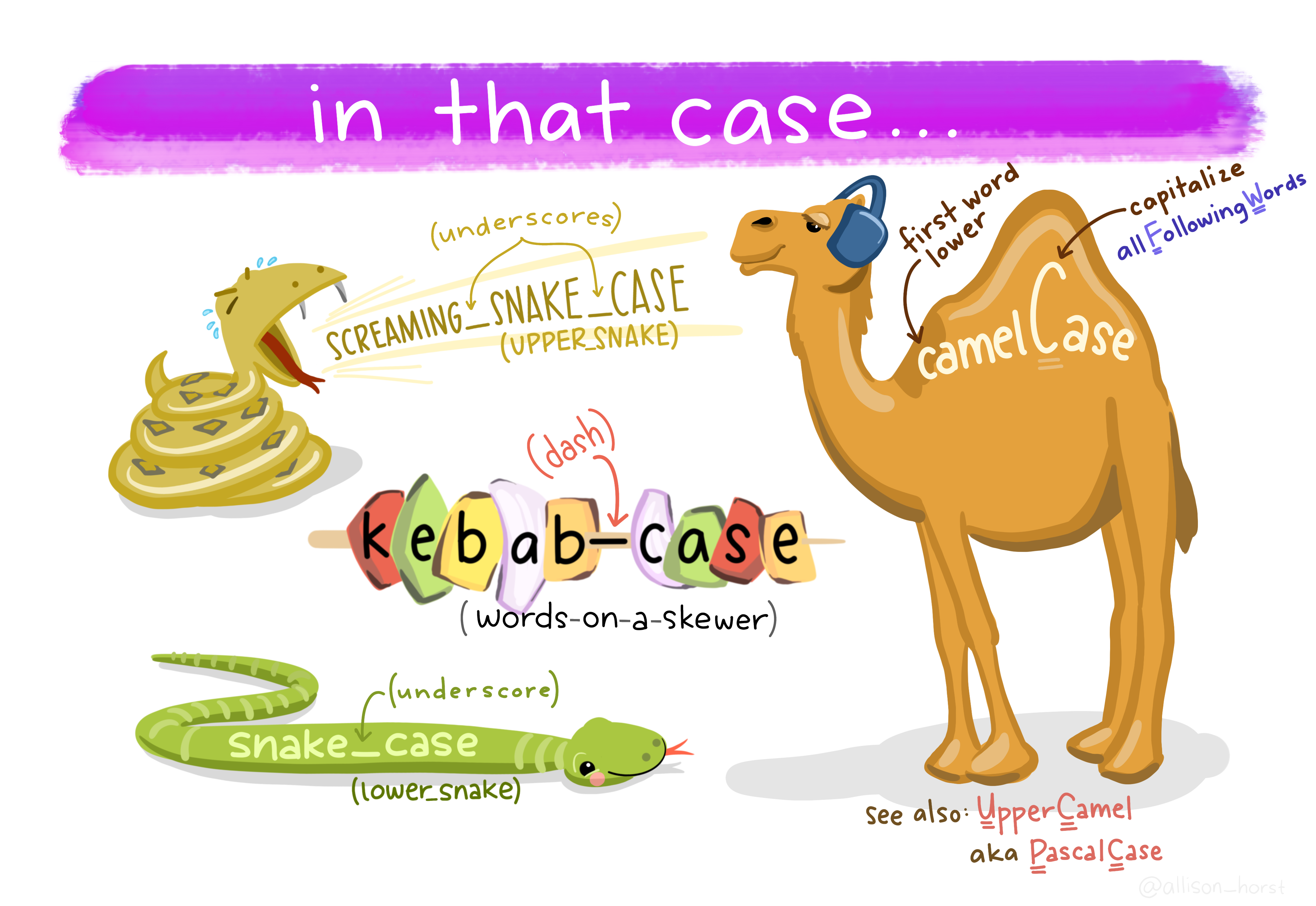
One important thing to do initially is develop a naming convention. This is important both for objects AND your files.
Object names must start with a letter, and can only contain letters, numbers, _ and .. File names require the same, but can also use -. However, you should avoid using . for both, and you should never use spaces! You want your names to be descriptive, so you will need a convention for multiple words.
Artwork by Horst (2022)
camelCase, where the first word is not capitalized and the first letter of each subsequent word is, is technically the most efficient in terms of keystrokes. You can run into some issues when using acronyms or singular letters (e.g., “RStudio” technically breaks this rule) though. More people have recently been recommending snake_case and arguing against the use of capital letters at all. Generally, only camelCase or snake_case are recommended.
You want to use names that are concise, unique, and meaningful (this is difficult!), avoiding terms that will be commonly repeated. This is also the case for your variable (column) and factor names as well. However, it IS helpful to develop a relatively consistent way of naming things for yourself. This helps make it easier to work with different projects (especially after some time). For example:
-
x_df – for dataframes
- Where “x” is refers to the type of data or your experiment
X_m – for the mean of some data
X_sd – for the SD of some data
X_se – for the standard error of some data
4.3.2 Style and Syntax
“Good coding style is like correct punctuation: you can manage without it, butitsuremakesthingseasiertoread.”
- Hadley Wickham
Many of the following tips are highlights from the tidyverse style guide.
4.3.2.1 Spacing
In general, you want to aim to write your code to be legible. This is both for your sake AND others. R makes no difference between the following code:
#1
3*2/2*5/2

((3 * 2) / 2) * 5 / 2

#2
x<-2+4

x <- 2 + 4- Always put a space after a comma, never before, just like in regular English:
# Good
df[, 1]

# Bad
df[,1]
df[ ,1]
df[ , 1]- Do not put spaces inside or outside parentheses:
- Most operators (
==,+,-,<-, etc.) should always be surrounded by spaces:
# Good
x + (3 * 4)

# Bad
x+(3*4)
4.3.2.2 Avoid Long Lines
Avoid writing code that takes up a lot of space horizontally. Use strategically placed line breaks and indentations, particularly after each argument/chunk of your code. You can use the keyboard shortcut cmd+i on OSX or ctrl+i on Windows to get R to automatically indent appropriately for you line-by-line!
# Good
do_something_very_complicated(
  something = "that",
  requires = many,
  arguments = "some of which may be long"
)

# Bad
do_something_very_complicated("that", requires, many, arguments,
                              "some of which may be long"
                              )
4.3.2.3 Misc.
Use double quotes
"hello", not single quotes'hello', for quoting text. The only exception is when the text already contains double quotes and no single quotes"She said, 'hello.'".Use
TRUEandFALSEoverTandFEach line of a comment should begin with the comment symbol and a single space:
#Index columns and subset rows by names or filtering, not numbers. Their order/position may change. Their name likely will not.
Pass named arguments into functions, not place.
DO NOT hardcode. Always softcode. It saves you from having to constantly update different sections of your code any time there is a change.
4.4 Pipes
This is a reference to René Magritte’s “The Treachery of Images,” which actually is on display at the LAC Museum of Art!
One of the more powerful tools in R that you will use is the %>% (pipe) operator.
RStudio Keyboard Shortcuts:
- OSX: CMD + SHIFT + M
- Else: CTRL + SHIFT + M
How Does a Pipe Work?
Consider the following example of making and eating a cake.
There are several things you need to do:
- Have ingredients
- Mix ingredients
- Pour mixture into pan
- Bake mixture
- Let cool
- Slice
- Eat a piece
One thing you might think to do is just go step by step:
mixture <- mix(ingredients)
thing_in_oven <- pour(mixture)
hot_baked_cake <- bake(thing_in_oven)
cooled_baked_cake <- cool(hot_baked_bake)
sliced_cake <- slice(cooled_baked_cake)

eat(sliced_cake, 1)
This creates a lot of unnecessary interim step variables that you do not care about. You will not use them again and they just clog up your workspace.
If you were to express this process as a set of nested functions, it would look like this:
eat(slice(cool(bake(put(pour(mix(ingredients), into = baking_pan), into = oven), time = 30), duration = 20), pieces = 6, 1))Nesting a dataframe inside a function is hard to read because it forces you to read the sequence of functions inside out. You have to start in the innermost parentheses, and then work your way out/back.
Even if you were to apply your style and syntax guidelines here:
eat(
  slice(
    cool(
      bake(
        put(
          pour(
            mix(ingredients),
            into = baking_pan),
          into = oven),
        time = 30),
      duration = 20),
    pieces = 6,
    1)
)
It is still difficult and unnatural to read. If you were to describe this process in words, spoken or written, it would take a totally different form! You might say something like:
“I need to start by taking my ingredients, mix them together, pour the mixture into a baking pan, and then put that pan into the oven and bake for 30 minutes. Once that is done let it cool for 20 minutes, slice into 6 pieces, and eat one of them (or several, if you are me)!”
It would be so much easier if you could write your code in a form that would match how you actually think about this process. That is precisely what piping with %>% allows you to do! Here is how you write this code with piping:
ingredients %>%
  mix() %>%
  pour(into = baking_pan) %>%
  put(into = oven) %>%
  bake(time = 30) %>%
  cool(during = 20) %>%
  slice(pieces = 6) %>%
  eat(1)
When you pipe a dataframe into a function, and chain together a number of functions, it lets you read left to right / up to down. Your code “sentence” starts with a noun instead of a verb. This is much easier to read and write because it takes the same form that you actually think about this process. It is in the chronological order of what you want to be doing.
There are two mantras with pipes:
- Think of a
%>%to mean “and then” - “dataframe first, dataframe once”
What the %>% operator is actually doing is taking the result/output of the previous computation (thing on the left or above) and piping it through as input to the next computation. In most cases, these computations will be functions.
mix(ingredients) is equivalent to ingredients %>% mix()
Below is an animated illustration of a similar example:
Source: Arthur Welle
4.4.1 Do’s and Dont’s
DO:
- Apply all the same style/syntax guidelines
- Space before and after a
%>% - Each new step on its own line
- Indent each subsequent line in a chain
- Etc.
- Space before and after a
DON’T:
Use a pipe when…
- More than one object needs to be manipulated.
- Pipes should only be used when a chain of steps is applied to one object.
- There are intermediate objects you need to use which could be given an informative name.
4.5 Data Importing and Exporting
While the built in datasets that R comes with can be very helpful, the whole point of learning R is to use it for our own needs. So you need some ways to get your raw data into R, and the products of your code out of R.
4.5.1 File Paths
A file’s path specifies where that file is located. It is like a map for your computer, giving it instructions on where to go to look for that specific file. When you download a file (e.g., “dataset.csv”), it likely would appear in your downloads folder. Thus, the full file specification would be:
For mac: /Users/user_name/Downloads/dataset.csv
For windows: C:\Users\user_name\Downloads\dataset.csv
(Replacing “user_name” with whatever the user name on your machine is)
A file path is constructed by 2 parts:
- the file location:
/users/user_name/Downloads/orC:\Users\user_name\Downloads\ - the file name:
dataset.csv
4.5.2 Importing
You are most often going to work with csv’s and .RData files. You can work with a number of other file types in R, but that will be beyond the scope of this class.
4.5.2.1 csv Files
You will use the read_csv() function to load a dataset into R. This function takes a file as its argument. How does R know where to look for the file? You need to give it the right file path!
# On mac
read_csv("/Users/user_name/Downloads/dataset.csv")

# On windows
read_csv("C:\Users\user_name\Downloads\dataset.csv")
If the output from read_csv() was not saved to a variable, it would just print it out in the console. You need a variable to get the output so you can use it later in your other code. You do this by saving it to a variable.
As an additional point, you can also directly load files from websites by using the website as the file path. Remember, a file path is just a map to tell your computer where to look for something. The file path just needs to lead read_csv() to a .csv file!
example_df <- read_csv("https://www.ethanhurwitz.com/example_data.csv")4.5.2.2 RData Files
The other type of file you may want to import is an .RData file. These directly load R objects into your workspace. Instead of using read_csv(), you just use load() and pass it the file path to a .RData file!
# On mac
load("/Users/user_name/Downloads/dataset.RData")

# On windows
load("C:\Users\user_name\Downloads\dataset.RData")
Since .RData files already contain R objects, you do not have to save this to a variable. It is loading variables that already exist!
4.5.3 Exporting
While the goal of using R code is to make your tasks easily reproducible, there are instances where you may want to directly save and export something. For example, you may want to use some data with other software. In these instances, you can easy export the file with write_csv(), which takes the form: write_csv(object_to_be_saved, file = "file_name.csv"). This will create a new .csv file of your dataframe/object in your working directory.
Alternatively, you may have run some code that takes a V.F.L.T. (Very, Frankly, Long Time) to run. Somewhere down the road you may be executing complicated models that can take hours or even days to run! You may not want to have to rerun this code consecutively each time you revisit that project. To avoid doing so, you can save R data object that you can easily load in to R.
You do so using the save() function, which takes a similar form of save(objects_to_be_saved, file = "fil_name.rdata").